Position sizing on a real bench: why our A/B can’t cleanly tell fixed from sigma

Once a strategy is written, the biggest open question is rarely which signal fires. It’s how much capital to commit when it does. That decision — position sizing — sets the geometric growth rate of the account, the drawdown profile, and the variance of returns far more than the choice of indicator.

This post compares three sizing rules used in the KreamEdge engine. They are not points on a ladder of sophistication; they target three different objectives:

1. Fixed fractional — assigns a fixed fraction of equity per entry. No objective beyond simplicity.
2. Kelly — maximises the long-run geometric growth rate of equity, conditional on the strategy’s per-bet edge and variance.
3. Sigma-targeting (inverse-vol) — sizes each position so that its ex-ante volatility contribution is the same. Targets equal risk contribution per name, not growth.

Sigma does not dominate Kelly in any well-defined sense — they answer different questions. The argument of this post is that under realistic operational conditions, the inputs Kelly needs are unavailable cheaply enough to matter, and sigma-targeting + a strong baseline (fixed) end up being the rules that actually survive contact with production.

This post also presents a multi-version A/B from the KreamEdge bench across four engine snapshots, isolating (a) flipping sigma on without changing anything else, (b) sigma + claimed reoptimisation, and (c) sigma + reopt + pruning the score weight vector. The cleanest finding is the third one — the others are weaker than a first-pass reading suggested, and this post is explicit about why.

---

1. Fixed fractional sizing

The simplest rule: every entry gets a fixed target weight w of equity. If w = 10 % and equity is 1 000 000, every new position is sized at 100 000 of notional. As equity grows or shrinks, so does the absolute bet size — this is geometric (compounding) sizing, not flat-dollar.

Pros

• One number, zero estimation error.
• Trivially auditable.
• Behaves well when you don’t know what you don’t know (small sample, regime shifts).

Cons

• Treats a 60 %-vol microcap the same as a 12 %-vol large cap. Risk contribution per position is wildly unequal.
• Ignores edge: an entry with a 0.9 expectancy gets the same size as one with 0.3.
• Drawdown is dominated by whichever subset of positions is the highest-vol at the moment.

Fixed sizing is the honest baseline. A lot of “Kelly improves things” claims in the trading literature fall apart when you replace the comparison with a properly tuned fixed-fractional run.

---

2. Kelly sizing — and why backtest-Kelly degenerates in practice

Kelly’s formula, in its log-utility, single-bet form:

f* = edge / variance

For a binary win/lose bet with win probability p and win:loss ratio b:

f* = (p·b − (1 − p)) / b

Apply this to a strategy whose backtest produced a pooled winrate p and average R:R b, and you get a single number. That number is constant across every signal — because the inputs are pooled statistics over the whole backtest. In the single-bet IID setting, backtest-Kelly reduces to fixed fractional sizing with a Kelly-implied scalar (p·b − (1 − p))/b. And because backtest p is typically biased high vs live p (slippage, missed fills, partial fills), that scalar is biased upward too. The shape collapses to fixed fractional; the size is systematically too aggressive.

Two caveats before that claim is taken too far:

• Multi-asset Kelly is not constant. With simultaneous bets and a real covariance matrix Σ, the growth-optimal weights are w* ∝ Σ⁻¹ μ. That’s genuinely state-dependent through Σ. The collapsing-to-a-constant argument only holds in the single-bet projection most retail blog posts assume. You still have to estimate μ and Σ from history, so the operational critique below applies, but the formula itself is not a scalar.
• “Fractional Kelly” (half, quarter) is principled, not a kludge. MacLean/Thorp/Ziemba (2011) show that when the standard error of your edge estimate is on the same order as the edge itself, the Bayes-optimal sizing is roughly half-Kelly. The shrinkage is the right response to known input noise — it is not “I gave up and picked a number.”

The reason backtest-Kelly hurts more than it helps in practice is input sensitivity. For a binary bet, ∂f*/∂p = (b + 1)/b. With b = 2, that’s 1.5. A 3-pt overestimate of winrate inflates f* by ~4.5 pts of equity. With b = 3, ~4 pts. Real systematic strategies routinely have winrate estimates with 3–5 pt standard errors over a 5-year backtest sample — which means full Kelly’s sample-driven error band swamps the signal.

Net: pooled-backtest Kelly is fixed fractional under a Kelly justification, with a scalar that’s biased toward over-leverage. Conditional Kelly is a genuinely different rule — per-signal edge estimates (signal-strength buckets, regime priors, slippage-adjusted live winrate) make f* state-dependent, and that conditioning is where its real edge lives. It is a defensible institutional choice when those inputs exist. Without them, what’s left is fixed fractional with extra paperwork: the input-sensitivity downside of Kelly without the conditioning upside.

---

3. Sigma-targeting (inverse-vol)

The rule: size each position so that its ex-ante volatility contribution to the portfolio is a fixed budget. Abstractly:

target_fraction = (daily_vol_budget_pct / 100) / sigma_daily

where sigma_daily is an EMA-smoothed std of daily returns of the underlying, captured at signal time, and daily_vol_budget_pct is the daily vol budget per name as a percent of NAV. A 0.25% setting means each new entry should contribute 0.25% of NAV in expected daily vol — roughly 4% annualised per name (× √252). High-vol names get smaller dollar bets, low-vol names larger ones.

Pros

• Equalises ex-ante risk contribution across names — drawdown is no longer dominated by whichever positions happen to be highest-vol right now.
• No per-signal edge estimation. The rule implicitly assumes equal Sharpe across names — a uniform edge assumption, but not a signal-by-signal one.
• Self-updating from market data: yesterday’s bars feed today’s vol estimate. No (p, b) lookup table to refresh.

Cons and traps

• Procyclical de-risking on V-bottoms. Vol expands during a correction → next entry undersized → recovery happens at small size → vol normalises just in time for the next correction. This is a real problem in equity books. Standard mitigations: longer estimation window, EWMA with a floor, capped target_fraction.
• The σ estimator is a hidden hyperparameter. Simple stdev, EWMA (RiskMetrics), GARCH, Yang-Zhang range, intraday realised vol — each gives different sizing. The 50-day EWMA stdev used in the KreamEdge engine is a defensible default for daily strategies — chosen for operational simplicity and estimator stability over reactivity — but it lags shock onsets. Yang-Zhang or GARCH react faster, at the cost of more noise in the size.
• Per-name vol-targeting is not portfolio-level vol-targeting. Ten correlated names sized at 4 %/yr each do not give a 12.6 % portfolio (√10 × 4 %). Cross-correlation in a sector squeeze can push that to 25 %+. The article’s bench, and KreamEdge’s live sizing, operate per-name; the gap to a true correlation-aware portfolio vol target is real and not closed here.
• More turnover. Vol estimates drift → target sizes drift → rebalancing trades. The bench data below quantifies this.
• Equal-edge assumption. If your highest-conviction signals also tend to fire on the most-volatile names, sigma sizing throws away signal information.

Sigma-targeting is the base layer most institutional systematic books run. The next layer up is risk parity / equal-risk-contribution at the portfolio level (correlation-aware), and the layer above that is a hard portfolio vol target combined with regime-conditional leverage. This post stays at the base layer because that’s what KreamEdge actually implements.

---

4. Operational profile: who pays the maintenance bill?

The theoretical comparison covers half the picture. The other half is the operational cost over the life of the system — and this is where Kelly is at its weakest.

Kelly’s two operational liabilities

(a) Inputs are not market-observable. p (winrate) and b (R/R) come from your historical fills + a backtest engine. That means:

• Refresh cadence. To stay calibrated, (p, b) need re-estimation periodically. Monthly is plausible; weekly is more defensible. Each refresh is a non-trivial pipeline (full OHLCV update, signal recomputation, simulated fills, statistics aggregation).
• Per-strategy maintenance scales linearly. KreamEdge’s bench carries 100+ strategies. That’s 100+ (p, b) pairs to keep fresh, each with its own backtest window choice, warm-up period, slippage assumption.
• Regime drift makes pooled (p, b) misleading. An 18-month bull-tape backtest produces p ≈ 60 %, b ≈ 2.5, and Kelly says size up. The first 6 weeks of a correction destroy that estimate, but Kelly under-sizes only after the rerun reflects the loss — by which time the damage is done. The same lag works against you on the way back up.

A clarification worth making explicit: refreshing an estimator is not the same as refitting parameters. If you only recompute (p, b) against new data without changing strategy parameters, you’re updating a statistic — that’s not data snooping. Snooping enters when you re-tune strategy parameters on the new data and then compute (p, b) from the re-tuned strategy. In practice almost everyone who reruns Kelly also reruns the optimiser, so the snooping case is the common one — but they are distinct operations.

There is a cleaner alternative: estimate (p, b) from rolling live fills, not from re-runs of the backtest. This is genuinely out-of-sample. Its weakness is statistical power — a strategy that fires 30 times a year cannot keep (p, b) calibrated fast enough to react to regime change. For institutional books that’s fine; for a one-person systematic shop it’s a deal-breaker for most strategies. There’s also a Bayesian/bootstrap variant — integrate over the posterior of (p, b) and size on the lower quantile — which is the principled answer to input uncertainty, but it requires non-trivial infrastructure.

(b) Live ≠ backtest. Backtested (p, b) come from idealised fills (mid-price, full size, instant). Live (p, b) include slippage, partial fills, missed orders, and the lag between signal and execution. The gap is always in the conservative direction — live edge is smaller. So even a perfectly-fresh backtest-Kelly is biased toward over-sizing. Note that fractional Kelly addresses the input-noise problem (MacLean/Thorp/Ziemba); it does not address the live-vs-backtest gap, which is a bias not a variance issue. That bias has to be closed separately, by validating slippage assumptions against live data periodically (which is another maintenance pipeline).

The net of (a) and (b): operating Kelly correctly means standing up infrastructure to refresh (p, b) per strategy on a fast cadence, validate slippage haircuts against live fills, and either run the live-fills version (which most retail shops can’t due to sample size) or accept some data-snooping cost from frequent re-optimisation. For a small systematic operation it almost always degenerates into “I ran a backtest in May and have been trading off those numbers since” — at which point Kelly has provided nothing fixed sizing wouldn’t.

Sigma-targeting: inputs are live and self-updating

Sigma uses realised volatility of the asset, computed from OHLCV. The properties that matter operationally:

• No backtest dependency. Yesterday’s bars become today’s vol estimate automatically. The DAL already has the data.
• Self-correcting under regime change (modulo procyclical-whipsaw caveat in §3). Vol expansion downsizes the next entry; no rerun required.
• Per-name, not per-strategy. The estimator is a property of the instrument, not the signal. Adding a strategy on the same universe doesn’t multiply the maintenance burden.
• One main hyperparameter: sigma_target_pct. Pick it once based on portfolio-level vol budget; review yearly. The σ estimator window/family is a second hyperparameter but is rarely changed once chosen.

The implementation reads the volatility estimate straight off the OHLCV pipeline at signal time and divides — no separate refresh job, no (p, b) lookup table, no “when did we last retune” question.

Fixed fractional: zero maintenance

Set w. Done. The only operational question is whether w is still appropriate for the current account size and risk appetite — a quarterly or yearly review at most.

Operational hierarchy

Rule	Inputs needed	Update cadence	Stale-input failure mode
Fixed	One number (w)	Yearly review	Suboptimal, never wrong
Sigma	Realised vol per name (live)	Automatic (rolling)	Bad if σ estimator broken; procyclical on V-bottoms
Kelly	(p, b) per strategy from backtest + slippage model	Monthly or faster	Over-sizing through regime changes; data-snooping if refits accompany refreshes

This operational gap is arguably the biggest reason Kelly underperforms in practice even when it would dominate in theory: the theory assumes inputs that are accurate and current; the operational reality is they’re stale and biased upward. Sigma and fixed sizing sidestep this — sigma because its inputs are market-observable, fixed because it has no inputs to maintain.

---

5. The A/B test: four engine snapshots on the KreamEdge bench

KreamEdge runs a strategy benchmark — a collection of optimised strategies across zones (Europe, US, Crypto, APAC), bar sizes, and base currencies. Each strategy carries a stable identifier, which makes it possible to track the same configuration across engine snapshots.

5.0 Caveats — read these before the numbers

This is a series of historical engine snapshots, not a designed experiment. The standing editorial position on backtest hygiene is set out in Why LLM Trading Backtests Are (Mostly) Nonsense, and a comparable matched-pair null-result write-up is the recent SPX market-regime filter analysis; the caveats below are the version of that hygiene applied to this specific bench. Three specific contaminations:

• The cost / financing model evolved within the bench window. During the four weeks the latest cohort was being assembled, the engine acquired a hedge-fund-style margin model (gross-exposure invariant + margin call), a refreshed short-borrow base rate, retuned retail-broker margin-spread caps, and a different default for borrow-fee accounting. Composite scoring was also retuned. Any matched-pair Δ between snapshots absorbs changes that have nothing to do with sizing. The early A→B and A→C deltas in particular include this drift, not just the sigma-flag change.
• Row selection uses the composite score. If the composite scoring formula changed between snapshots (it did, at least once), “best composite” picks different rows on each side. Manual inspection confirmed the same stable IDs survived, but the winning configuration within that name may differ across snapshots for non-sizing reasons.
• No multiple-comparisons correction. Five metrics × four contrasts = twenty hypothesis tests; none of the bootstrap CIs below are corrected for multiplicity. Read the headline findings as patterns across metrics, not as isolated significance claims.

So the bench is suggestive about the direction and rough magnitude of effects, not a precise unit-tested measurement of sigma vs fixed. Treat the numbers as evidence in a chain of arguments, not as causal estimates.

5.1 The four snapshots

Snapshot	Sizing rule	Score weights	Notes
A	Fixed fractional	16-element score vector, optimised	Baseline
B	Sigma, 0.25% daily-vol budget	Same as A (sigma flag flipped only)	Sizing-only change
C	Sigma, 0.25–0.40% budget	Same as A on legacy rows; 21 new rows freshly optimised	“Reopt” was partial
D	Sigma, 0.40% budget (mostly)	11 weights (5 pruned) + retuned	Full retune + score pruning

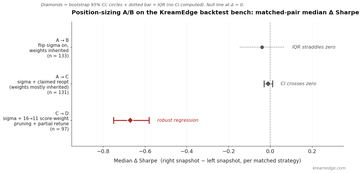
Pairs are matched by stable strategy ID; the row with the highest composite score per side is taken. All Δ figures are (R − L) per strategy. Bootstrap CIs are 2 000-sample percentile intervals on the median.

5.2 A → B: flip sigma on, weights inherited (n = 133)

All 133 matched rows had identical scoring weights to A. The optimiser did not run; only the sizing flag changed.

Metric	Median Δ	IQR	Bootstrap 95 % CI (median)
CAGR	−0.79 pts	4.0	—
maxDD	0.00	4.0	—
Sharpe	−0.04	0.21	—
Sortino	−0.07	0.32	—
R/R	−0.32	0.85	—

This is the cleanest isolation of “sizing only” in the bench, and the central estimate is small and slightly negative. The IQR straddles zero on every metric; this is not a sigma-helps or sigma-hurts result at the single-strategy median — it’s a no obvious effect on weights-tuned-for-fixed.

5.3 A → C: claimed reopt (n = 131 matched + 21 new)

The C batch was supposed to be “sigma + reoptimised”, but checking the weight vectors row-by-row:

• 130 of 131 matched names still had unchanged weights. The optimiser did not actually rerun on those.
• Only 1 matched row had genuinely retuned weights.

The matched-pair deltas are correspondingly small:

Metric	Median Δ	IQR	Bootstrap 95 % CI (median)
CAGR	−0.30	4.24	[−0.71, −0.01]
maxDD	−0.17	3.96	—
Sharpe	−0.01	0.19	[−0.03, +0.01]

The bootstrap CI on median ΔSharpe crosses zero; the CI on median ΔCAGR is narrow but barely negative ([−0.71, −0.01]) — functionally flat. The Sharpe-level finding is not statistically distinguishable from noise; the CAGR-level finding is marginal at best. An earlier framing called this “essentially flat — sigma has no effect when weights are inherited”; that’s directionally right, but overstated the precision.

The 21 strategies new in C, optimised from scratch under sigma sizing, look much better than the A baseline (median CAGR 25.7 vs 17.4; median Sharpe 1.16 vs 0.67). Two reasons to handle this carefully:

1. Selection bias. A fresh optimiser run produces best-of-N survivors. The 21 are the best of a fresh search; the A baseline is an aged cohort. Comparing them is “best of fresh search under sigma” vs “median of historical cohort under fixed” — that conflates sizing changes with search-vintage. The honest comparison is a fresh optimiser run on the same universe under fixed sizing, head-to-head with a fresh run under sigma. That comparison has not been run.
2. In-sample only. All numbers are on the optimisation window. A held-out drift check on the 21 new rows is the next step.

So the claim “freshly-optimised sigma strategies are materially better than the legacy fixed-sized cohort” is real in the data but not cleanly attributable to sigma yet. A more conservative read: fresh optimisation under sigma produces good strategies; whether they’re better than fresh optimisation under fixed is open.

5.4 C → D: sigma + score-weight pruning 16 → 11 + retune (n = 97 matched)

All 97 matched rows had changed weight vectors, so the optimiser genuinely ran. This is also where the bench data is strongest:

Metric	Median Δ	IQR	Bootstrap 95 % CI	Strategies that improved
CAGR	−4.12	6.99	[−5.54, −3.20]	24 / 97
maxDD	+8.35	10.91	—	7 / 97 (i.e., 93 % got worse)
Sharpe	−0.67	0.60	[−0.75, −0.58]	5 / 97
Sortino	−1.02	0.67	—	3 / 97
Winrate	−4.14	—	—	—
#Trades	+94 (~2×)	194	—	—

This regression is wide and statistically robust: bootstrap CIs are tight and far from zero; only 5 of 97 matched strategies improved on Sharpe. Whatever changed between C and D hurt the existing strategy cohort badly.

The new strategies in D (n = 14), optimised from scratch under the 11-weight engine, look fine on their own (median CAGR 24.8, maxDD 16.3, Sharpe 0.74). So the 11-weight engine can produce good strategies — but the legacy strategies, retuned only on weights and not re-searched on signal combinations, regressed sharply.

This post will not single out any one weight as the load-bearing one; the bench cannot prove which of the 5 pruned weights mattered. Several competing explanations are not ruled out by the data:

1. One or more pruned weights were doing real risk-control work.
2. The retune changed the remaining 11 weights but kept the signal-combination and stop-level parameters fixed — that’s a partial reopt, not a full re-search.
3. The cost/financing model changed in the same window (margin model, borrow base, composite coefficient — all listed in §5.0). Some of the regression is plausibly attributable to honest cost models making previously-overstated returns shrink.
4. Optimiser search budget may differ between snapshots.

A clean ablation would re-run D but with all 16 weights restored — to separate the pruning effect from the composite/cost retune. That ablation hasn’t been run yet. The defensible headline is the empirical one: pruning + partial-retune produced a broad regression, not a particular causal claim about which weight matters.

5.5 Exposure-adjusted return — sharpens the picture

If sigma sizes positions smaller, a like-for-like CAGR comparison is misleading. Computing return per unit of average gross exposure (CAGR / exposure %):

Snapshot	Median CAGR / exposure
A (fixed)	34.3
C (sigma, ~inherited weights)	36.2
D (sigma, 11-weight retune)	30.1

On this measure, C is marginally better than A — sigma achieves the same CAGR per unit of exposure as fixed, possibly slightly better, but at a lower absolute exposure. That’s a more defensible reading of the A → C step than “sigma is neutral or slightly worse”: when you control for gross exposure, sigma roughly matches fixed and the lower headline CAGR is because the book is running smaller.

D’s regression survives this normalisation — it’s worse in both raw and exposure-adjusted terms — which strengthens the §5.4 conclusion.

5.6 Summary across the four snapshots

Change	Empirical finding	Confidence
Flip sigma on, keep weights (A → B)	Small negative median, IQR straddles 0	Not distinguishable from noise
Sigma + claimed reopt that was actually inherited weights (A → C)	CAGR median Δ in [−0.71, −0.01]; Sharpe Δ in [−0.03, +0.01]	Marginal at best; matched fixed on exposure-adjusted return
Sigma + freshly-optimised strategies (21 new in C)	Materially better than baseline (CAGR +8, Sharpe +0.5)	Real but confounded with selection bias (fresh-search advantage)
Score pruning 16 → 11 + partial retune (C → D)	CAGR −4, Sharpe −0.7, DD +8	Robust; CIs tight

The strongest defensible finding is the last one: structural engine changes (here: pruning the score vector) require a full re-search of strategy parameters, not just a weight retune. That’s an engineering lesson, not a sizing one.

On sizing itself, the bench supports a weaker claim than the earliest reading suggested: sigma sizing is roughly exposure-equivalent to fixed sizing when weights are tuned to fixed, and possibly better when allowed to co-optimise — but the “possibly better” case is contaminated by selection bias. A clean head-to-head fresh-optimisation A/B is needed to settle it.

---

6. Practical takeaways

For a single, well-characterised strategy with a stable edge starting from scratch: fixed fractional is the honest baseline. It’s robust to estimation error, and the fraction can be sized by judgement or half-Kelly intuition. The KreamEdge bench’s matched-pair A → C result — Sharpe Δ indistinguishable from zero, exposure-adjusted return slightly up — is consistent with this: at the single-strategy level the choice between fixed and sigma is a wash, so the simpler rule wins.

For a basket of strategies on a basket of names with very different volatility profiles (single names + ETFs + crypto in the same book), sigma-targeting is the right base layer on theoretical grounds — it equalises ex-ante risk contribution across heterogeneous names — and a portfolio-level vol target belongs on top of it, because per-name vol-targeting ignores cross-correlation and will under-budget gross exposure during sector squeezes. The bench in §5 does not isolate this benefit empirically, since the strategies in it are single-instrument; the basket recommendation rests on theory, not on the bench. The KreamEdge engine doesn’t run the correlation-aware layer yet; that’s an open piece.

Anyone reaching for Kelly should answer two questions before starting. First: what conditional estimate of edge per signal is the input? If the answer is “the pooled backtest winrate”, that’s fixed sizing under a Kelly justification, not Kelly. Second: how does (p, b) stay calibrated — by re-running the backtest (with the data-snooping cost that re-tuning the strategy introduces) or by estimating from rolling live fills (which requires enough fills per strategy per period to be statistically meaningful)? Without a concrete pipeline for the second question, Kelly will be stale within a quarter and will be doing damage by the next regime change.

And when the score vector or any other structural piece of the engine changes, re-run the full optimisation — including signal-combination search, not just weight retuning. Snapshot D pruned 5 of the 16 score weights, retuned the remaining weights, and produced a flat-out regression on 93 % of legacy strategies. The 11-weight engine isn’t broken — strategies started from scratch under it look fine — but its loss surface is different enough from the 16-weight one that legacy strategies can’t recover by re-weighting alone. The signal combinations and stop levels need to move too, and that’s not what the retune did.

The least defensible position is that a sizing rule, a score formula, or a cost model can be changed independently of the others. They’re coupled through a single loss surface. The KreamEdge bench shows that empirically.