The hidden bias in long backtests
Every strategy that screens for sufficiently liquid stocks uses a threshold: only trade names where average daily value traded clears some minimum floor. That filter exists for good reasons. Thin stocks are expensive to trade and hard to model accurately. But it hides a distortion when applied over a long backtest window.
Nominal dollar volume is not stationary. Over a fifteen-year window, broad market growth means that a stock of equivalent relative liquidity generates significantly more dollar volume at the end of the period than at the start. A flat threshold calibrated to today’s market is much harder to clear in 2010 than in 2026. The practical effect: the backtest skips valid entries in early years, or narrows the eligible universe to only the largest names that cleared the bar even then. The in-sample period ends up structurally narrower than today’s live runs. Not because the strategy logic changed. Because the eligibility filter behaved differently over time.
This is a form of survivorship bias built into the liquidity filter itself. It operates silently: no error, no warning, just fewer signals in the early part of the window and a biased universe selection in later years.
The fix: a time-varying floor anchored to SPX growth
The solution is to scale the eligibility threshold over time instead of holding it flat. The S&P 500 acts as a proxy for broad market nominal growth. If the SPX’s 200-day moving average has grown fourfold since 2010, then a stock of equivalent relative liquidity back then would have traded at roughly one-quarter of today’s dollar volume. Scaling the threshold down by the same factor restores consistent behaviour across the full window. The gate is as strict in 2010 as it is today, measured in relative terms.
The key design question is where to apply the scaling. The obvious approach is to adjust the value-traded data itself: divide each bar’s dollar volume by the scale factor. The correct approach is to leave the data untouched and scale the threshold instead, bar by bar. At each point in time the gate asks: does this stock’s actual, nominal dollar volume clear a floor that has been proportionally relaxed relative to the current SPX level? The result is identical either way. The implementation is not, and the difference matters for everything downstream.
Why scaling the data fails
The first implementation scaled the value-traded series at source. Two bugs surfaced in review.
The first was execution contamination. Value-traded data feeds more than the eligibility gate. It also informs the slippage model and the borrow-cost model. When the series was deflated at source, those downstream calculations inherited the scaled values. Early-year trades appeared far cheaper to execute than they actually were: slippage and borrow costs in 2010 were computed against deflated liquidity, not against real historical conditions. The backtest looked better in the early period for the wrong reason.
The second problem was that the scale factor depended on where the backtest window ended. Extending the end date by a few months shifted the reference level and retroactively changed which historical bars cleared the eligibility gate, including bars well inside the in-sample period. That violates a core requirement of walk-forward research: pushing the out-of-sample boundary forward must not alter past results. The first version failed that test.
The gate-side approach
The revised implementation keeps value-traded data strictly nominal throughout. The scaling is applied only to the eligibility floor: at each bar, the threshold is the configured minimum multiplied by the ratio of the SPX 200-day moving average at that bar to its value at the end of the loaded window. Early in the backtest the floor is lower; at the latest bar the scale is approximately 1.0 and the floor matches the configured minimum exactly. The gate flexes over time. The underlying data, and every metric computed from it, remains unchanged.
The 200-day moving average is used rather than the raw SPX close to avoid crash-driven artefacts. A sharp equity drawdown would relax the liquidity floor at precisely the moment when real liquidity is most impaired. That is the opposite of the intended behaviour. A smoothed level removes that spike without changing the long-run trajectory.
The SPX level is computed once across the full window and applied identically to every symbol. If each symbol recomputed its own moving average, stocks listed on non-US exchanges with different holiday schedules would see slightly different scale factors, creating differences in the eligible universe across otherwise identical runs. A single precomputed series eliminates that divergence.
Limitations of the SPX deflator
The SPX 200-day moving average is a practical choice. It is not the right deflator for every situation, and three limitations are worth naming explicitly.
First, it is US-equity-centric. For strategies trading non-US equities or multi-asset instruments, the SPX trend may not accurately capture local liquidity growth. A regional index or a total market cap series would be more representative. For this strategy, which targets liquid equities with broad exposure to global benchmarks, SPX is a reasonable stand-in, but it is not neutral.
Second, there is a residual look-ahead in the normalization. The scale factor at each historical bar is computed relative to the SPX level at the end of the loaded window. A 2010 bar is normalized against a 2025 reference that did not exist in 2010. A fully clean implementation would anchor the scale to a fixed reference date rather than the window endpoint. The effect here is small and its direction is conservative, but it is a form of forward bias.
Third, the SPX captures one source of non-stationarity: broad nominal market growth. It does not model changes in market microstructure, exchange fee structures, or shifts in institutional participation that also affect practical liquidity thresholds over time.
The main virtue is simplicity. One observable series, one ratio, no additional data dependencies. As a first-order correction to a documented bias, that trade-off is acceptable.
What this means for signals and results
At the latest bar, the one that drives today’s screener output, the SPX scale is approximately 1.0. The eligibility threshold matches the configured floor, and the live signal universe is unchanged. Users receiving strategy output today will not see any difference in which names appear.
For historical backtests, the update expands the eligible universe in early years and removes the execution contamination that made early-period trades appear artificially cheap. Benchmark files generated before this change should be regenerated before any direct comparison with post-update runs. The two are not comparable on historical bars, and treating them as equivalent would produce misleading conclusions.
The legacy flat-threshold behaviour is preserved and reproducible via a run flag. This makes it straightforward to isolate the effect: run both modes on the same universe and compare fills directly. The legacy mode is intended for controlled A/B analysis, not for ongoing production runs.
Bottom line
- A flat value-traded threshold is stricter in early backtest years than at the current bar. It silently narrows the early-period universe and introduces a structural bias into long-window results.
- The fix scales the eligibility floor proportionally to broad market growth, using the SPX 200-day moving average, without modifying value-traded data or any downstream execution metric.
- The SPX deflator is a practical first-order fix: simple, observable, and no extra data dependencies. It is US-equity-centric, carries a residual look-ahead from anchoring to the window endpoint, and does not model microstructure changes. Acknowledge those limits before applying it to non-US or multi-asset strategies.
- Live screener signals at the current bar are unaffected; the scale at that point is approximately 1.0.
- Historical benchmark files must be regenerated before comparing to new runs; pre-update and post-update results on historical bars are not directly comparable.
- The legacy flat-threshold mode remains available for controlled isolation of the effect.
This strategy’s rules and parameters were frozen on 3 July 2025; all performance after that date is genuine out-of-sample / forward-tracked data, unseen at selection time, with no hindsight possible. All results discussed here are from backtests run under controlled conditions with realistic cost modelling, no look-ahead bias, and explicit in-sample/out-of-sample separation. Past backtest performance does not guarantee future results. This post is informational and educational, not financial advice.
Methodology questions or comments? Join the discussion via the KreamEdge community channels.
0 Comments